How to Read Age on a Pedigree
During the Exploratory Data Analysis or EDA phase one of the key things you'll want to do is sympathize the statistical distribution of your information. Histograms are one of the quickest and easiest fashion to achieve this, since they group together numeric data into bins to provide a simplified representation of the data.
The functionality for plotting them is congenital direct into Pandas. However, technically, the histograms and other data visualisations in Pandas aren't actually produced past Pandas itself. Instead, Pandas provides a wrapper to the Matplotlib PyPlot library which gives you quick access to the main features of PyPlot, without the need to write all of the underlying code.
The out-of-the-box functionality for visualisations using the Pandas wrapper doesn't allow you lot to practice everything in a one-liner, but you can practise most things, and you can easily add together any missing functionality by utilising Matplotlib code on top of the Pandas functions. Here's how information technology's done.
Load packages
Nearly of the things we're looking at here tin exist done using solely the Pandas library. However, as we may need to call Matplotlib and Numpy, nosotros'll load these packages too.
import pandas as pd import numpy every bit np import matplotlib.pyplot as plt Load data
I've used the Pima Indians diabetes dataset here, as it contains a skilful mix of information. You tin download this from diverse places, including the UCI Machine Learning Repository. It's a good thought to tidy up the cavalcade names upon import and to driblet the row of original cavalcade headers, which aren't formatted nicely for use with Pandas.
df = pd . read_csv ( 'diabetes.csv' , names = [ 'meaning' , 'glucose' , 'bp' , 'skin_thickness' , 'insulin' , 'bmi' , 'full-blooded' , 'age' , 'outcome' ], skiprows = one ) df . caput () | pregnant | glucose | bp | skin_thickness | insulin | bmi | pedigree | age | outcome | |
|---|---|---|---|---|---|---|---|---|---|
| 0 | half-dozen | 148 | 72 | 35 | 0 | 33.6 | 0.627 | l | i |
| i | i | 85 | 66 | 29 | 0 | 26.half dozen | 0.351 | 31 | 0 |
| 2 | 8 | 183 | 64 | 0 | 0 | 23.3 | 0.672 | 32 | 1 |
| 3 | ane | 89 | 66 | 23 | 94 | 28.one | 0.167 | 21 | 0 |
| 4 | 0 | 137 | 40 | 35 | 168 | 43.ane | 2.288 | 33 | ane |
Creating a histogram of a specific column
To create a histogram of a specific column or Series from our Pandas dataframe nosotros tin can append the .hist() function later defining the dataframe and cavalcade name. By default, this gives the states a histogram with a standard size and colour and no title, with data spread across 10 bins. This gives us a good view of where glucose levels lie within the data.
glucose = df . glucose . hist () 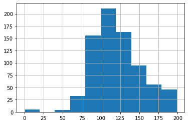
Changing the histogram size
To change the size of the standard histogram we can add the figsize() argument and pass in a tuple of values. The first one is the width in inches (how quaint), and the second is the acme in inches.
glucose = df . glucose . hist ( figsize = ( 16 , 4 )) 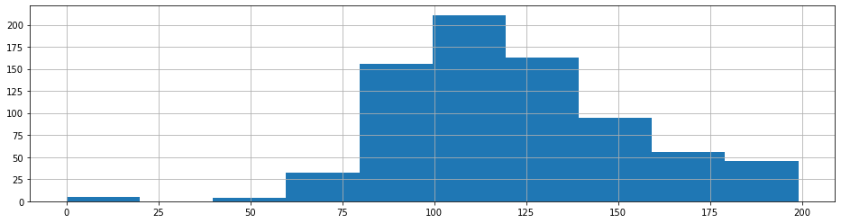
Calculation a title to the histogram
To add a championship yous can suspend set_title() and pass in a cord value. There's more yous can practise with titles, such every bit changing the size and weight of the font, simply you need to practise this using Matplotlib.
glucose = df . glucose . hist ( figsize = ( vii.two , 4 )). set_title ( 'Glucose' ) Irresolute the number of bins
The standard histogram defaults to 10 bins, however, you can alter the number of bins by passing an integer to the bins statement of the hist() role. Setting bins to 100 gives a more granular view of the data.
glucose = df . glucose . hist ( figsize = ( 7.two , iv ), bins = 100 ). set_title ( 'Glucose' ) 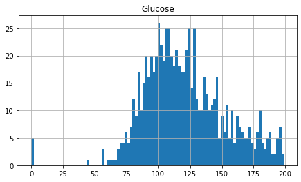
Turning off the grid
If you want a more minimalist view of your data yous can plow off the grid lines by passing in the Simulated to the filigree statement, which is set up to True by default.
glucose = df . glucose . hist ( figsize = ( 7.2 , 4 ), filigree = Fake ). set_title ( 'Glucose' ) 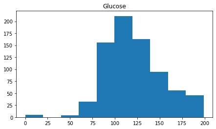
Changing the colour of histograms
By default, Pandas histograms are dark blueish, but you lot can define a custom colour by passing in a color value. This can either be a named colour cherry or orangish, or information technology can be a specific hex code, similar #32B5C9.
glucose = df . glucose . hist ( figsize = ( 7.2 , four ), color = "orange" ). set_title ( 'Glucose' ) 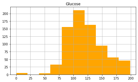
age = df . historic period . hist ( figsize = ( vii.2 , 4 ), color = "#32B5C9" ). set_title ( 'Age' ) 
Adding border colours to histograms
If you want to make the distinction betwixt each bar in your histogram a flake more distinct, you can laissez passer in a colour value to the ec statement which changes the edge colour. Here's the chart higher up with the grid turned off and the edge colour set to white.
age = df . age . hist ( figsize = ( 7.ii , 4 ), colour = "#32B5C9" , ec = "white" , filigree = False ). set_title ( 'Age' ) 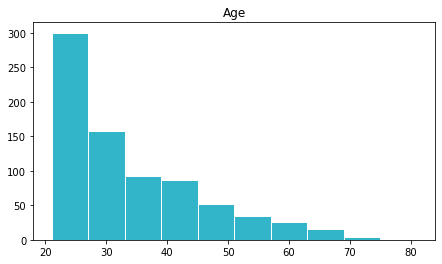
Changing histogram orientation
By default, Pandas histograms are displayed vertically, but you tin can change this to horizontal past passing in the optional argument orientation='horizontal' to the hist() function.
glucose = df . glucose . hist ( figsize = ( seven.ii , 4 ), orientation = 'horizontal' ). set_title ( 'Glucose' ) 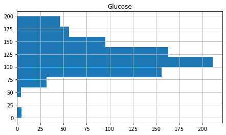
Creating histogram subplots
To view the statistical distributions of all of the numeric columns in your dataframe, instead of passing in a specific cavalcade, you can provide the entire dataframe. Pandas volition automatically create a unmarried chart with a subplot for each of the numeric columns. In the beneath case, I've manually defined the figure size and then information technology fits the width of the page.
histograms = df . hist ( figsize = ( 16 , 8 )) 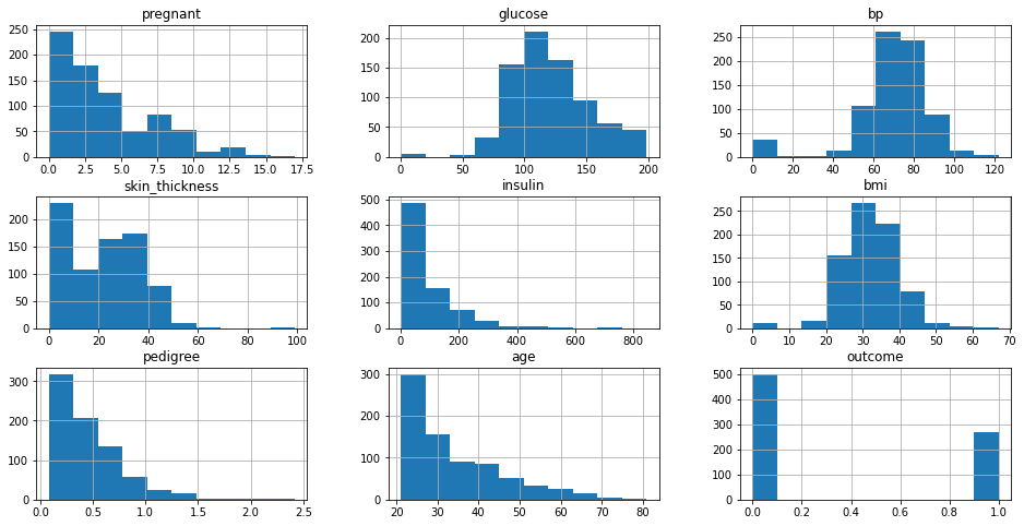
Selecting specific data for subplots
If you desire to view two or more specific histogram subplots of your numeric data you'll need to bring in a little Matplotlib lawmaking. Firstly, we'll apply the subplots() office of PyPlot to create a figure containing 1 row and 2 columns, with a full size of 16 inches past 4 inches. Then we'll create two histograms as nosotros did above, but nosotros'll ascertain which position they occupy on ax by passing in axes[0] for the left column and axes[1] for the correct.
fig , axes = plt . subplots ( i , 2 , figsize = ( 16 , 4 )) glucose = df . glucose . hist ( ax = axes [ 0 ]). set_title ( 'Glucose' ) outcome = df . age . hist ( ax = axes [ 1 ]). set_title ( 'Diabetes' ) 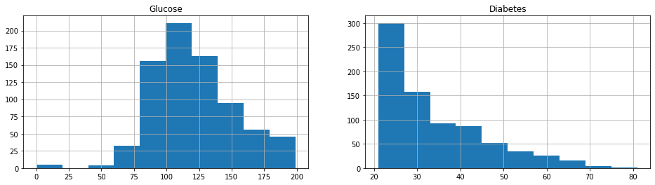
It'southward easy to echo this process for the more than ii histograms, of class. Simply change the number of subplots from ane,two to one,iii and add an additional histogram to be displayed in position axes[two].
fig , axes = plt . subplots ( one , 3 , figsize = ( sixteen , 4 )) age = df . historic period . hist ( ax = axes [ 0 ]). set_title ( 'Age' ) glucose = df . glucose . hist ( ax = axes [ 1 ]). set_title ( 'Glucose' ) upshot = df . age . hist ( ax = axes [ two ]). set_title ( 'Diabetes' ) 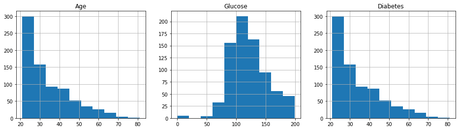
Creating stacked histograms
If you have two columns of data that share the same unit of measure, y'all can plot them on a stacked histogram by passing in the argument stacked=Truthful. There's no data like that in this dataset, so hither'south a completely nonsensical example, simply to show you what it looks like.
df [[ 'glucose' , 'insulin' ]]. plot . hist ( stacked = True , bins = 10 , figsize = ( 7.2 , 4 )) 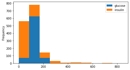
Advanced styling
Y'all can combine some of the approaches above with some boosted Matplotlib lawmaking to achieve some more stylish designs. In the example below I've added the rwdith=0.ix argument to increase the width between the bars, and have passed in some extra arguments to hibernate the spines, remove the title, and add some larger axis labels.
ax = df . hist ( cavalcade = 'glucose' , bins = 10 , grid = False , figsize = ( 16 , eight ), color = "#32B5C9" , rwidth = 0.ix ) ax = ax [ 0 ] for ten in ax : 10 . set_title ( "" ) ten . set_xlabel ( "" , labelpad = thirty , weight = 'assuming' , size = 13 ) ten . set_ylabel ( "Glucose" , labelpad = 30 , weight = 'bold' , size = 13 ) x . spines [ 'correct' ]. set_visible ( False ) x . spines [ 'height' ]. set_visible ( False ) 10 . spines [ 'left' ]. set_visible ( False ) 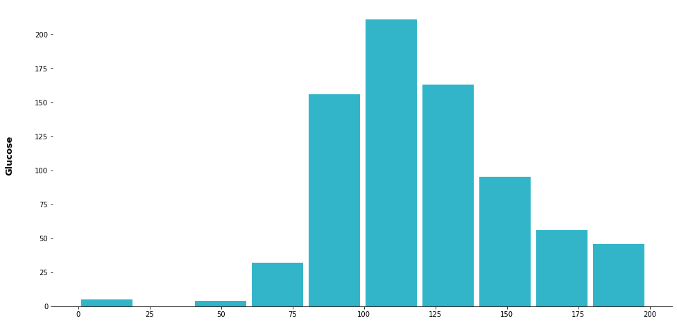
Matt Clarke, Saturday, March 06, 2021
Source: https://practicaldatascience.co.uk/data-science/how-to-visualise-data-using-histograms-in-pandas
0 Response to "How to Read Age on a Pedigree"
Post a Comment